Time is arguably one of the most critical concepts in any application, especially in distributed ones: Setting timeouts, measuring performance, caching, logging, and most other operations require some measurement of time to operate. Time works intuitively in a single-threaded application, where one operation happens after the other. However, in distributed systems, where processes might run concurrently and without a physically synchronous global clock, it becomes a real challenge to measure time and track events’ order. In this post, we will explore Physical and Logical clocks, the algorithms for implementing them, and their role in distributed systems.
Physical Clock
Physical clocks measure time in seconds, and all processes have access to physical clocks based on vibrating quartz crystals. Quartz clocks are cheap, though they are not entirely accurate due to manufacturing defects and the external temperature, and these factors can make such clocks run faster or slower than others.
The rate at which a clock runs (fast or slow) is called drift, and the difference between two clocks at a specific time is called skew.
Another more accurate physical clock is an atomic clock which measures time based on the resonance frequencies of atoms. Atomic clocks are highly precise however they are too expensive and bulky to replace Quartz clocks so, to solve the issue of drifting, Quartz clocks are synchronized with atomic clocks from time to time using the Network Time Protocol (NTP). At the core, NTP utilizes a clock discipline algorithm to adjust an NTP client’s clock time based on the time received from an NTP server.
Every mainstream operating system comes with an NTP client built-in.
Time synchronization using NTP might seem trivial on the surface but in practice, this is far from the truth - network latency and node inaccuracies can make this a challenging feat. Thus a combination of selection and filtering algorithms are used to achieve accurate time synchronization.
Using the NTP, a client can adjust its time to the most accurate time, however, this solution introduces a substantial flaw - the adjustment of time by the client can cause the clock to jump forward or backward in time which makes the measurement of time error-prone, for example, we might record inaccurate execution time of an operation due to drift.
Physical clocks drift, as such, most operating systems offer monotonic clocks. These clocks guarantee that no sudden jumps will happen. Unlike physical clocks, a monotonic clock does not measure time in the sense of current date or time, instead, it starts counting from some arbitrary moment, for example, the moment an operation begins. A monotonic clock aids with computing the elapsed time between two events observed on a single node.
The downside of a monotonic clock is that it is only suitable for measuring elapsed time on a single node. Computing monotonic clock timestamps across different nodes in a distributed system would not make much sense.
Logical Clock
In a distributed system, we look at time from a different angle. Instead of measuring time in seconds, we focus on accurately capturing the order of events. Formally, this is known as logical clock.
To understand logical clocks, let’s first look at an idea in computer science called happens-before relation. Happens-before is a relation that assumes, given two events, when one happens before the other, the output of the events must reflect this relationship. For example, if event e1 sends a message to event e2, then the message sent by e1 must have happened before it is received by e2 (e1 -> e2).
This is a partial order, it is possible for some event e1 to have happened neither before nor after another event e2. In such case we assume e1 and e2 to be concurrent (e1 || e2).
By concurrent, we do not mean e1 and e2 happened at the same time, instead we assume that e1 and e2 are independent events.
Now that we understand the happens-before relationship, let’s look at our first logical clock, Lamport clock.
Lamport Clock
A Lamport clock is a counter, responsible for counting the number of events that occurred and incrementing the counter with each occurrence. Each node in a distributed system has its own local Lamport counter, and the counter is incremented each time an operation is executed. When a node communicates with another node (for example when sending a message), the sender would attach its local Lamport counter with the message, and the receiver would increment its counter when the message is received.
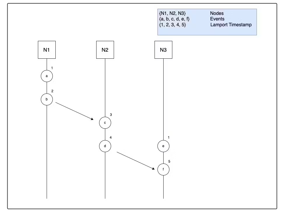
The Lamport clock guarantees that if an event a happened before an event b, then b will always have a greater Lamport timestamp than a. The limitation of the Lamport clock is that the converse of this property is not true, i.e. if the timestamp of an event a is lower than the timestamp of another event b, then it is not possible to know if a actually happened before b or if they are concurrent.
In our diagram, we can see that event e has a lower timestamp than c but e did not happen before c. In this case, this implies that event e and c does not have a happens-before relationship i.e. they are concurrent (e || c).
In the above case, we had information about all the events in all three nodes, so we were able to determine that c || e, however, suppose, if we are only given two Lamport timestamps, a and b, and a is less than b, then we cannot really determine if a happened before b (a -> b), or if they are concurrent (a || b). In many cases, it would be useful to have this information, and for this reason, we have another logical clock called vector clock, which lets us determine if events are concurrent.
Vector Clock
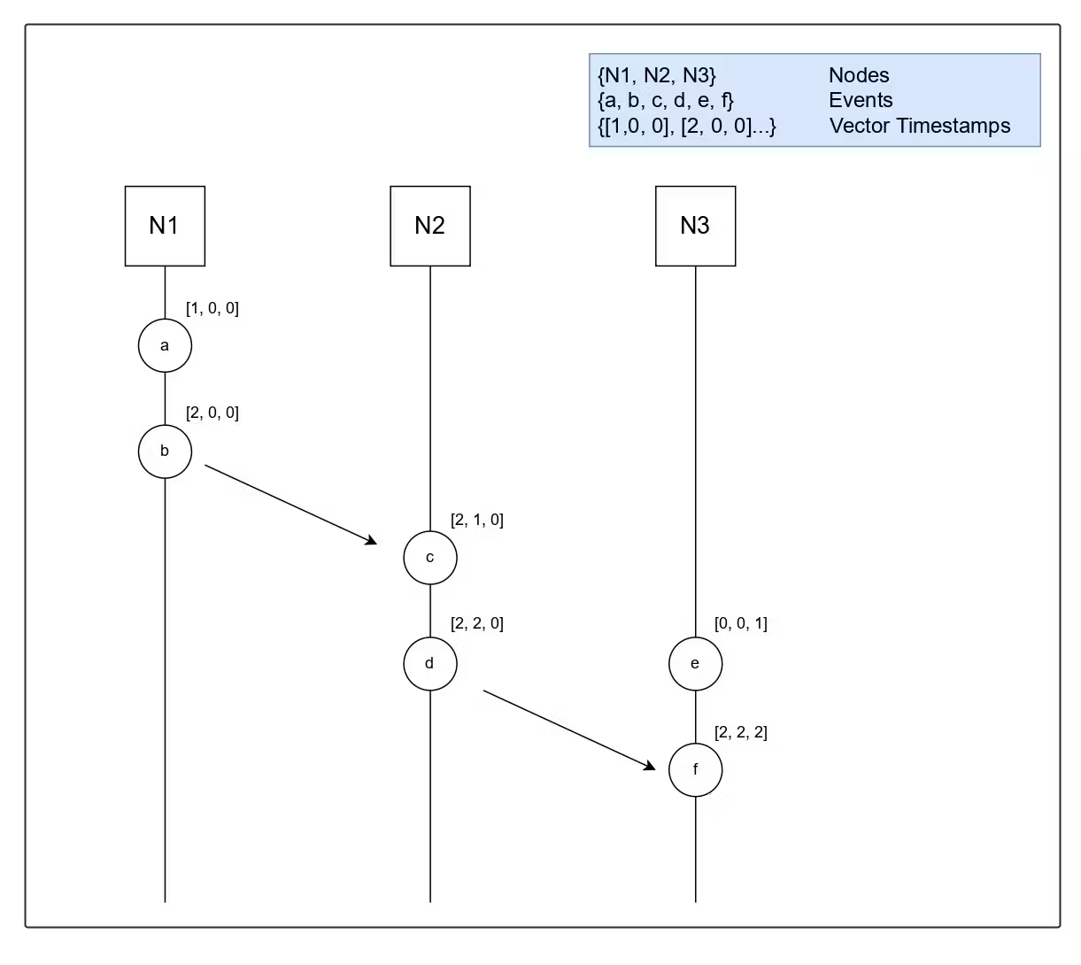
Vector clock is similar to Lamport clock, in the sense that both employ counters - In a Lamport clock, we have a single counter, whereas in a Vector clock we have an array of counters. Let’s understand vector clocks with an example, suppose there are three nodes in a distributed system N1, N2, and N3. Each node will have a vector timestamp implemented as [ tN1, tN2, tN3 ], where tN1, is the timestamp for N1, tN2 is the timestamp for N2 and so on. Initially, each timestamp in the array is set to 0, and when an operation executes on a node, the timestamp corresponding to that specific event is incremented by 1.
In our example, when N1, sends a message to N2, N1 would increment the timestamp tN1 by 1, and attach a copy of its array with the message. When N2 receives the message, it would merge its local array with the copy sent by N1 by taking the element-wise maximum of two arrays and then incrementing its own timestamp. The diagram below should aid in understanding this algorithm.
With Vector clocks we can define a partial order. The rules for defining this order are -
Given we have two events E1 and E2, with tE1, and tE2 as the arrays of their vector timestamps.
If every timestamp in tE1 is less than or equal to the corresponding timestamp in tE2, and there is at least one timestamp in tE1 lower than tE2, then E1 -> E2.** In our diagram, b -> c**.
If we cannot meet the above requirements, then the events are considered to be concurrent. In our diagram, c || e.
This wraps up our discussion of time and clocks in distributed systems. The concept of time can feel a bit abstract, but it forms the basis of distributed systems, and recognizing different types of clocks would aid us in the journey of understanding distributed systems.